Motion Planning Library

After creating a Studio Project that appropriately represents your use application and use case. You can then use that project in your code in order to quickly generate bold, collision free, and singularity free motions using the Motion Planning Library.

Basic Motion Library Structure

The Motion Planning Library is a collection of classes that will help you get the motions you need for your project. The basic class structure of the library is as follows:

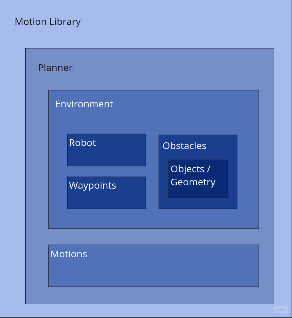
Class Object Overview

Planner

The Planner is the primary object that you will be interacting with. It contains wrapper functions that simplify all the motion planning work you may want to do with your robot. The planner also holds all the data structures necessary for you to perform more complex motion planning, as well as manipulate the robot and it’s environment.

For more details on the Planner you can visit the Python or C++ Documentation

Environment

The Environment class holds all of the data related to the environment, it also contains a Robot object. This class allows for the planner to be able to check for collisions and plan around them.

When imported from a jacobi project created in studio, any Obstacles and Waypoints created in studio can be extracted from the Environment object for future use.

For more specific details on Environment you can visit the Python or C++ Documentation

Robot

The Robot class holds all information about the robot’s kinematics, operating limits, as well as link and end-effector geometries. Each supported robot arm is instantiated based off of it’s robot type name. You can find a full detailed list of those robots in our Python or C++ Documentation.

This class is where you will set robot operation settings such as the speed of the robot and limits; as well as generate forward or inverse kinematics between joint and cartesian space.

Tip

💡 Don’t see the robot you want in our supported list? You can create a custom robot using the CustomRobot class. Simply supply a custom .urdf that represents your robot.

Obstacles

Obstacles are a series of classes that represent physical geometry that you might use in your robot workcell. An obstacle can be represented as the following basic geometry Object:

PythonC++

box = Box(x = 1,y = 2,z = 3)
capsule = Capsule(radius = 1, length = 2)
cylinder = Cylinder(radius = 1, length = 2)
sphere = Sphere(radius = 1)

To create an Obstacle object, use a basic geometry Object and a Frame in order to give the appropriate origin of the Obstacle.

PythonC++

obstacle = Obstacle(box, Frame(x = 0,y =0,z =0)

Obstacles can also be custom meshes for more complex applications. Using convex allows for you to upload a mesh file using load_from_file(). Currently the Jacobi Motion Library takes in stl, obj, and blg files for loading custom meshes with convex

PythonC++

convex = Convex.load_from_file('path_to_3d_mesh')
obstacle = Obstacle(convex, Frame(x = 0,y = 0,z = 0)

For more specific details on Obstacles you can visit our Python or C++ Documentation

Waypoints & Cartesian Waypoints

Waypoints represent points in space of importance that the robot can reach. Each Waypoint contains position, velocity, and acceleration information of the robot’s joint configuration at that point. A Waypoint constructer is overloaded such that if a velocity and acceleration are not given, they will default to 0.

When creating waypoints in code, other than normal waypoints, you can also create a CartesianWaypoint. A Cartesian Waypoint will have a reference_config along with the the position, velocity, and acceleration of the robot in Cartesian Coordinates. The reference_config class variable is a joint configuration used in reference when planning a motion to that point. If a Cartesian Waypoint has a defined reference_config then any motion planned with it will deterministically use that joint configuration at that Cartesian Waypoint.

PythonC++

joint_position = [-3.702, -1.907, -1.796, 0.898, 0.337, 0.524]
tcp_position = Frame(x = 0.458,y = 0.235,z = 0.456)

wp1 = Waypoint(joint_position)
wp2 = CartesianWaypoint(tcp_position, reference_config = joint_position)

Once a waypoint is defined, as long as there is a collision free path to that waypoint and it is within the robot’s reach, a robot can plan to that waypoint from it’s current position.

For more details on Waypoints you can visit our Python or C++ documentation

Using the Motion Library

While it is possible to perform all the actions of setting up a planner, creating waypoints, and planning motions programatically, the motion library is meant to be used in conjunction with Studio. We recommend that a typical development cycle take studio into account and program with with a downloaded jacobi project from studio.

Creating a Planner & Extracting Important Information

When programming with the Jacobi Motion Library you must first create a Planner object, from which you will be able to extract all the necessary information needed for planning motions.

PythonC++

#creating a planner from a jacobi project
planner = Planner.load_from_project_file('path to your jacobi project')
environment = planner.environment
robot = environment.get_robot()

p1 = environment.get_waypoint('waypoint1')
p2 = environment.get_waypoint('waypoint2')

box1 = environment.get_obstacle('Box 1')
box2 = environment.get_obstacle('Box 2')

Tip

💡 Planner does have a manual constructor such that you would have to separately create an environment, and a robot object as inputs in order to create a Planner that way.

Planning Motions

Planning motions using the Jacobi Library is easy! As long as you have set up your planner object, and have set waypoints for your robot to go to, all you have to do is:

PythonC++

trajectory = planner.plan(p1, p2)

The result of the plan function is a trajectory that begins at your given start waypoint and ends at the goal waypoint. This trajectory can be used to control your robot either through our robot drivers or as a trajectory input anywhere else it is needed.

---

There are a few ways that you can choose to plan your motions for your robot applications. We recommend that when in an application setting, motions are computed based off of the current position of the robot, to the desired final waypoint.

PythonC++

current_pose = robot_driver.current_joint_position
next_trajectory = planner.plan(current_pose, p2)
robot_driver.run(next_trajectory)

It is important to remember the type of waypoint used to plan a motion will determine the results of the motion you plan. For example if you planned a motion with a CartesianWaypoint that has a reference_config set, then you can deterministically have your robot arrive at a given joint configuration.

Manage Your Environment

When executing your robot application, your environment will change as your robot executes it’s task. It is important to make sure that the changes in environment are concurrent with the planner, this will allow your robot to be able to accurately and safely plan around static obstacles. The simplest way to perform environment management is to add and remove static obstacles in your environment as they appear or change.

PythonC++

#create a box obstacle with its origin at a given frame
box = Obstacle(Box(0.3,1,0.2), Frame(x = 0.432, y = 0.013, z = 0.588))
environment.add_obstacle(box)

#removing the obstacle from the environment
environment.remove_obstacle(box)

Tip

💡 Any motions that are planned before editing the environment will need to be planned again to take into account a change in the environment. This is another reason why we recommend planning motions as needed for execution time.

Tip

💡 When visualizing obstacles don’t forget to call the studio function studio.add_obstacle()as well in order to make sure your obstacle appears in the the visualizer in Studio Live

Adding End Effectors and End Effector Obstacles

Adding end effectors and end effector obstacles using the motion library is done via the robot class. End Effectors as well as obstacles that may be attached to end effectors are class variables of robot . When setting the end effector don’t forget to also set the appropriate transformation from the robot flange to the new TCP using the flange_to_tcp function.

An end effector can also be set using either representative geometry or using your own meshes. The Jacobi Motion Library currently is able to accept stl obj and glb 3d file formats.

PythonC++

robot.end_effector_obstacle = Convex.load_from_file('project path to 3d mesh')
robot.flange_to_tcp = Frame(x = 0.1, y = 0.1, z = 0.3)

Tip

💡 In the same way as a change an environment requires pre-planned motions to be re-planned. A change to the robot’s end effector, and end effector obstacle’s would need motions to be planned with that change in mind. This is another reason why we recommend planning motions as needed at execution time.